Algorithm analysis

Algorithm analysis is the practice of measuring how much computing resources — time and memory — an algorithm uses, as a function of its input size. It lets you compare algorithms abstractly, before any code is written, by counting basic operations rather than running the program with a stopwatch.

The result of analyzing an algorithm is a time function $T(n)$: the number of basic operations the algorithm performs on an input of size $n$. From $T(n)$ you typically extract a Big O bound that describes the function’s growth rate.

Axioms of basic operations

The standard set of “basic operations,” each assumed to take constant time:

1. Memory access — fetching or storing an integer takes $T_{\text{fetch}}$ or $T_{\text{store}}$. So y = x + 1 takes $T_{\text{fetch}}+T_{\text{store}}$.
2. Arithmetic and comparison — add, subtract, multiply, divide, compare integers, all constant. y = y + 1 takes $2T_{\text{fetch}}+T_{\text{op}}+T_{\text{store}}$.
3. Function calls — call and return are constant ($T_{\text{call}}$, $T_{\text{return}}$). Passing an integer argument is one fetch.
4. Array subscripting — computing the address of a[i] takes constant time $T_{[]}$, not including the time to compute i or to fetch/store the element.
5. Memory allocation — for analysis purposes, malloc is treated as constant $T_{\text{new}}$ (excluding initialization). In reality, malloc is only amortized constant under specific allocator assumptions. A free-list-based allocator can hit the slow path on a request that needs to grow the heap (mmap/sbrk syscall, possibly hundreds of microseconds), and an arena allocator’s resize-and-copy fallback is even worse. The constant-time assumption is fine for big-O analysis but breaks down when you care about latency tails or when you’re measuring real-time behavior.

To simplify, set all these to 1 clock cycle: $T=1$. Then the time function counts the number of basic operations.

Frequency-count method

Count how many times each statement executes, multiply by its per-instance cost, sum up.

Example: sum the elements of an array.

int sum(int a[], int n) {
    int s = 0;                   // 1 store         → 1
    for (int i = 0; i < n; i++) {   // n+1 compares → n+1
        s = s + a[i];            // n iterations × const → n
    }
    return s;                    // 1 fetch          → 1
}

Total: $T(n)=2n+3$.

The dominant term grows linearly with $n$, so $T(n)=O(n)$.

Worst case, average case, best case

For algorithms whose running time depends on the contents of the input, not just its size, three quantities matter:

• Worst case $T_{\text{worst}}(n)$: the maximum running time over all inputs of size $n$. Usually what we care about.
• Average case $T_{\text{average}}(n)$: the expected running time over a random input. Often more informative for practical performance.
• Best case $T_{\text{best}}(n)$: the minimum. Usually less interesting except as a sanity check.

Example: searching for a value in an unsorted array. Worst case: scan the whole array, $O(n)$. Best case: the value is in position 0, $O(1)$. Average case: scan half the array, $O(n)$ (still linear).

Worked example: find maximum

int FindMaximum(int a[], int n) {
    int result = a[0];                       // line 3
    for (int i = 1; i < n; ++i)              // line 4
        if (a[i] > result)                   // line 5
            result = a[i];                   // line 6
    return result;                           // line 7
}

Counting per line:

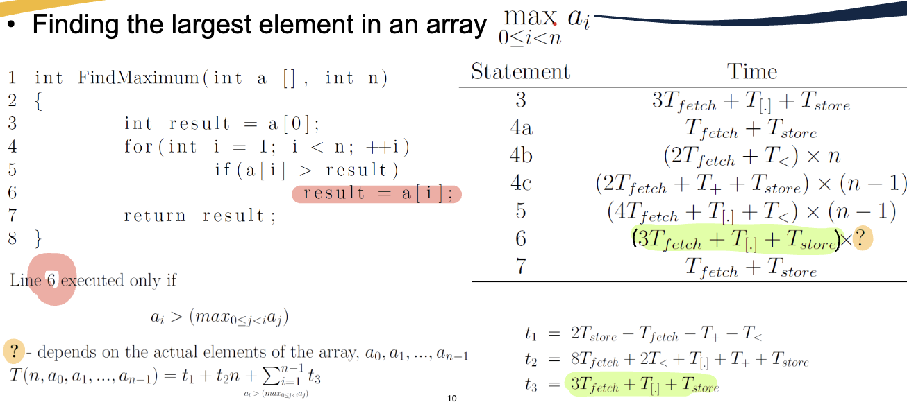
The wrinkle: line 6 only executes when $a_i>{\max }_{0\le j<i}{a}_j$ — depends on the actual data. So $T(n)$ has a data-dependent term that varies between best, worst, and average cases.

For average case on random inputs: the probability that $a_i$ is the largest seen so far is $\frac{1}{i+1}$. Summing across all $i$ gives:

$T_{\text{avg}}(n)=t_1+t_{2}n+t_3{\sum }_{i=1}^{n-1}\frac{1}{i+1}$

The harmonic sum is $O(\log n)$, so the average case is dominated by the $t_{2}n$ term: still $O(n)$.

For worst case: line 6 always fires (input is sorted ascending). $T_{\text{worst}}(n)=(t_1-t_3)+(t_2+t_3)n=O(n)$.

For best case: line 6 never fires (the first element is already max). $T_{\text{best}}(n)=t_1+t_{2}n=O(n)$.

All three are $O(n)$ — the constant differences don’t affect the asymptotic class.

Why we don’t track exact constants

For comparing algorithms, exact constants don’t matter — they’re determined by the hardware, the compiler, the workload. What matters is how the running time scales with input size. An $O(n^2)$ algorithm will eventually beat an $O(n\log n)$ algorithm, no matter how generous the constants. We use Big O notation to capture this scaling and ignore constants.

For the formal Big O machinery, see Big O notation. For the cost models specific to each algorithm, see the individual algorithm notes.