Bounce diagram

A bounce diagram is a graphical method for tracking voltage and current waves bouncing back and forth on a Transmission line when a transient (DC step, pulse, or other non-sinusoidal signal) is applied. It’s the time-domain counterpart to the standing-wave analysis used for sinusoidal steady state.

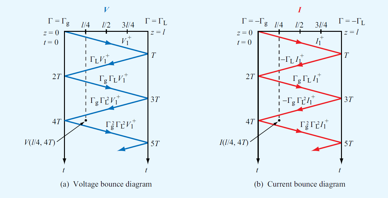Bounce diagrams: voltage (left) and current (right). The line at $z=0$ is the generator end, $z=l$ is the load end. Time flows downward. Diagonal lines show waves bouncing between the two ends with reflection coefficients ${\Gamma }_g$ and ${\Gamma }_L$ at each reflection.

Setup

A transmission line of length $l$, characteristic impedance $Z_0$, connected at $z=0$ to a generator $V_g$ with source impedance $R_g$, and at $z=l$ to a load $R_L$.

Define one-way travel time:

$T=\frac{l}{u_p}.$

Reflection coefficients at each end (treating the source and load as terminating impedances):

${\Gamma }_g=\frac{R_g-Z_0}{R_g+Z_0},{\Gamma }_L=\frac{R_L-Z_0}{R_L+Z_0}.$

These tell you what fraction of an incident voltage bounces back from each end.

How the diagram works

Time goes downward on the vertical axis; position $z$ along the horizontal. The line traces out the trajectory of each wavefront:

1. At $t=0$: the switch closes and the source launches a forward wave $V_1^{+}$ at $z=0$. During the first transit ($0<t<T$), no reflection has yet returned from the load, so the source sees only the line’s characteristic impedance $Z_0$ — not $R_L$. The launched amplitude is the voltage divider between $R_g$ and $Z_0$: $V_1^{+}=\frac{V_g{Z}_0}{R_g+Z_0}.$ This formula is valid only for $t<2T$ at the source end, before the first reflection returns. After that, the source sees a superposition of the incident wave it’s still launching and the returning reflected wave.

2. Forward wave travels at $u_p$: it arrives at $z=l$ at $t=T$.

3. At $t=T$: the load reflects. Reflected amplitude is $V_1^{-}={\Gamma }_L{V}_1^{+}$. This wave travels back.

4. At $t=2T$: the reflected wave reaches the source. Some fraction reflects again (at the source mismatch): $V_2^{+}={\Gamma }_g{V}_1^{-}={\Gamma }_g{\Gamma }_L{V}_1^{+}$. This launches a new forward wave.

5. At $t=3T$: $V_2^{+}$ reaches the load. Reflects: $V_2^{-}={\Gamma }_L{\Gamma }_g{\Gamma }_L{V}_1^{+}={\Gamma }_g{\Gamma }_L^2{V}_1^{+}$.

And so on. Each “bounce” multiplies the amplitude by another factor of ${\Gamma }_g$ or ${\Gamma }_L$.

Reading voltage at a specific point

To find $v(z_0,t_0)$ for a given $(z_0,t_0)$:

1. Locate the point $(z_0,t_0)$ on the bounce diagram.
2. Sum the amplitudes of all forward and backward waves that have passed over that point before time $t_0$.

Each wave contributes its amplitude (positive or negative depending on sign of ${\Gamma }_L,{\Gamma }_g$). Once a wave passes, it stays “contributing” — it doesn’t reset. The voltage at any point is the sum of all incident-plus-reflected waves through that point at that time.

Worked example

A line with $Z_0=100$ Ω, length $l$, generator $R_g=4Z_0$, load $R_L=2Z_0$. Switch closes at $t=0$ with DC source $V_g$.

Reflection coefficients:

${\Gamma }_L=\frac{2Z_0-Z_0}{2Z_0+Z_0}=\frac{1}{3},{\Gamma }_g=\frac{4Z_0-Z_0}{4Z_0+Z_0}=\frac{3}{5}.$

Initial launched wave:

$V_1^{+}=\frac{V_g{Z}_0}{4Z_0+Z_0}=\frac{V_g}{5}.$

Wave amplitudes over time:

• $V_1^{+}=V_g/5$ (forward, launched at $t=0$).
• $V_1^{-}={\Gamma }_L{V}_1^{+}=V_g/15$ (reflected from load at $t=T$).
• $V_2^{+}={\Gamma }_g{V}_1^{-}=V_g/25$ (re-reflected from source at $t=2T$).
• $V_2^{-}={\Gamma }_L{V}_2^{+}=V_g/75$ (reflected from load at $t=3T$).
• …

After many round-trip times, the voltage on the line settles to a steady-state DC value determined by the resistive divider:

$V_{\text{steady}}=V_g\cdot \frac{R_L}{R_g+R_L}=V_g\cdot \frac{2Z_0}{4Z_0+2Z_0}=\frac{V_g}{3}.$

This must equal the sum of the geometric series of bounces:

$V_{\text{steady}}=V_1^{+}(1+{\Gamma }_L+{\Gamma }_L{\Gamma }_g+{\Gamma }_L^2{\Gamma }_g+\dots )=\frac{V_1^{+}(1+{\Gamma }_L)}{1-{\Gamma }_L{\Gamma }_g}=\frac{V_g/5\cdot 4/3}{1-1/5}=\frac{V_g/3}{\cdot }✓.$

The bounce diagram is an alternative way of summing this infinite series — useful for visualizing the transient, but the algebraic geometric-series approach gives the answer directly.

Pulse propagation

A rectangular pulse of duration $\tau$ launched from the source becomes two step-shaped wavefronts: one rising step at $t=0$, one falling step at $t=\tau$. Each independently bounces on the diagram. Their sum at any point gives the actual voltage.

For $\tau <T$: the pulse fits within one transit time and arrives at the load as a distinct pulse, then reflects.

For $\tau >T$: the pulse is partially on the line and partially still being launched when the reflection arrives — the front of the pulse is reflecting from the load while the back is still being launched.

This is the basis of time-domain reflectometry (TDR): send a pulse down an unknown line, observe the reflections to characterize impedance mismatches, faults, or load impedances. Reflection arriving at time $2T_n$ pinpoints a discontinuity at $z=u_p{T}_n$.

In context

The bounce diagram is for the time domain what the Smith chart is for the frequency domain. Same physics, different problems:

• Bounce diagram: transient response to step/pulse inputs. Useful for digital signaling, switching circuits, lightning surge analysis.
• Smith chart: steady-state response to sinusoidal inputs. Useful for RF matching, antenna design, microwave components.

Both rely on the same underlying reflection coefficient $\Gamma$ — just deployed differently.