Electric potential

The electric potential $V$ at a point is the work per unit positive test charge required to move that charge from a reference point (usually infinity) to the given point, against the Electric field:

$V=-{\int }_{\text{ref}}^P\mathbf{E}\cdot d\mathbf{l}\text{(V)}.$

Equivalently, the potential difference between two points is

$V_{21}=V_2-V_1=-{\int }_{P_1}^{P_2}\mathbf{E}\cdot d\mathbf{l}.$

Units: volts (V), defined so that one joule of work moves one coulomb of charge through one volt: $1\text{V}=1\text{J/C}$.

Why a potential exists

The line integral $\int \mathbf{E}\cdot d\mathbf{l}$ is path-independent in electrostatics. This is the property that makes $V$ a single-valued function of position. Equivalently:

${\oint }_C\mathbf{E}\cdot d\mathbf{l}=0,$

the closed-loop integral of $\mathbf{E}$ is zero. By Stokes’ theorem this is the same as

$\nabla \times \mathbf{E}=0\text{(electrostatic case)}.$

A field with zero curl is a Conservative vector field; it is the gradient of a scalar. We define the scalar so that

$\mathbf{E}=-\nabla V.$

The minus sign is a convention: $\mathbf{E}$ points “downhill” from high to low potential, the same way a ball rolls.

In time-varying problems, $\nabla \times \mathbf{E}=-{\partial }_t\mathbf{B}\ne 0$ from Faraday’s law, so the scalar potential alone isn’t enough and a vector potential is also needed. That’s why $V$ is a clean concept in electrostatics but more subtle in dynamics.

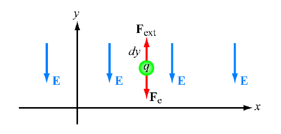Work done by an external force moves a positive charge against $\mathbf{E}$, raising its potential.

Potential of a point charge

A charge $q$ at the origin. From Coulomb’s law $\mathbf{E}=(q/4\pi ϵR^2)\hat{\mathbf{R}}$, with reference at infinity ($V_{\infty }=0$):

$V(R)=-{\int }_{\infty }^R\frac{q}{4\pi ϵR^{\prime 2}}d{R}^{\prime }=\frac{q}{4\pi ϵR}.$

So potential falls off as $1/R$ (slower than $\mathbf{E}$‘s $1/R^2$).

For a charge at ${\mathbf{R}}_1$, observation point at $\mathbf{R}$:

$V(\mathbf{R})=\frac{q}{4\pi ϵ|\mathbf{R}-{\mathbf{R}}_1|}.$

Superposition

For multiple charges:

$V(\mathbf{R})=\frac{1}{4\pi ϵ}{\sum }_{i=1}^N\frac{q_i}{|\mathbf{R}-{\mathbf{R}}_i|}.$

This is a scalar sum, not a vector sum, a big practical advantage over computing $\mathbf{E}$ directly. Compute $V$, then take $-\nabla V$ to get $\mathbf{E}$ if needed.

For continuous distributions:

$V(\mathbf{R})=\frac{1}{4\pi ϵ}\int \frac{{\rho }_v({\mathbf{R}}^{\prime })}{|\mathbf{R}-{\mathbf{R}}^{\prime }|}d{v}^{\prime }.$

Same form for ${\rho }_s$, ${\rho }_l$.

Equipotential surfaces

Surfaces of constant $V$. Since $\mathbf{E}=-\nabla V$ and gradients are perpendicular to level surfaces, $\mathbf{E}$ is everywhere perpendicular to equipotential surfaces.

A perfect conductor in electrostatic equilibrium has $\mathbf{E}=0$ inside, so $V$ is constant throughout: a conductor is an equipotential body. Its surface is an equipotential surface, and the external $\mathbf{E}$ just outside is perpendicular to it.

Worked example: ring of charge

A circular ring of radius $a$ in the $xy$-plane, line charge density ${\rho }_l$. Find $V$ at $(0,0,z)$ on the axis.

Every infinitesimal element $d{l}^{\prime }=ad{\varphi }^{\prime }$ is at distance $R^{\prime }=\sqrt{a^2+z^2}$ from the field point, the same for all ${\varphi }^{\prime }$.

$V=\frac{1}{4\pi {ϵ}_0}{\int }_0^{2\pi }\frac{{\rho }_{l}ad{\varphi }^{\prime }}{\sqrt{a^2+z^2}}=\frac{{\rho }_{l}a}{2{ϵ}_0\sqrt{a^2+z^2}}.$

To get the on-axis $\mathbf{E}$, take the gradient (only ${\partial }_z$ contributes by symmetry):

$E_z=-\frac{\partial V}{\partial z}=\frac{{\rho }_{l}az}{2{ϵ}_0(a^2+z^2{)}^{3/2}}.$

Direct integration of Coulomb’s law for $\mathbf{E}$ would have required vector components and cancellations by symmetry. The potential approach is much cleaner.

Poisson and Laplace equations

Combining $\nabla \cdot \mathbf{D}={\rho }_v$ with $\mathbf{D}=ϵ\mathbf{E}$ and $\mathbf{E}=-\nabla V$:

${\nabla }^{2}V=-\frac{{\rho }_v}{ϵ}\text{(Poisson’s equation)}.$

In a charge-free region, this reduces to

${\nabla }^{2}V=0\text{(Laplace’s equation)}.$

These PDEs determine $V$ in a region from the boundary data (the potential on the boundary, or the field at the boundary). Once $V$ is known, $\mathbf{E}=-\nabla V$ everywhere.