Generalization (machine learning)

Generalization is a model’s ability to perform well on data it has never seen during training. It is the purpose of supervised learning: fitting the training set perfectly is trivial but useless if the model fails on every new input. Every methodological choice in ML (test splits, regularisation, cross-validation, hyperparameter tuning) exists to estimate or improve generalization.

A model trained on data drawn from some underlying distribution $\mathcal{D}$ doesn’t really care about its loss on the specific training samples. It cares about its expected loss on a fresh sample from $\mathcal{D}$, the true risk or generalization error:

$R(\theta )={\mathbb{E}}_{(x,y)\sim \mathcal{D}}[L(f_{\theta }(x),y)].$

We can never measure $R(\theta )$ exactly because we don’t have all of $\mathcal{D}$. We approximate it with the training risk (loss on training data) during fitting, and with the test risk (loss on held-out data) when we evaluate.

Generalization gap

The generalization gap is the difference between training and test performance:

$\text{gap}=R_{\text{test}}-R_{\text{train}}.$

A small gap means the model performs about as well on new data as on training data: it generalizes. A large gap means the model has memorised training-specific patterns that don’t transfer, so it overfits.

Three regimes capture the typical shape:

• Underfitting. Both training and test losses are high. The model isn’t expressive enough or hasn’t trained long enough. Generalization gap is small but performance is bad across the board.
• Good fit. Training loss is low, test loss is also low, gap is moderate. The model captures genuine signal.
• Overfitting. Training loss is very low (or zero), test loss is much higher. The model has memorised noise and idiosyncrasies of the training set. Gap is large.

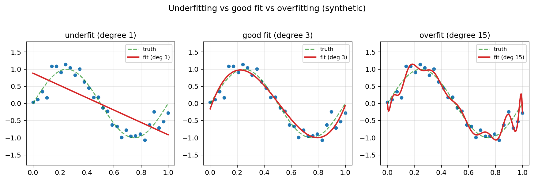Underfit / good fit / overfit on the same synthetic data — high-degree polynomials chase noise.

The classical U-shaped curve: as model capacity grows from too-simple to too-complex, training loss decreases monotonically, but test loss decreases then increases. The bottom of the test-loss U is the optimal capacity, high enough to capture signal, low enough to avoid memorising noise.

Why a model with low training loss can still generalize badly

A model with enough parameters can memorise anything: the underlying pattern in the data, plus the specific noise in the training samples. Any new sample drawn from the same distribution will have different noise, so the memorised noise is useless and probably harmful for predictions.

Concretely: a 10-degree polynomial fit to 11 noisy samples passes through every sample exactly (training loss = 0). On a fresh sample, the polynomial’s wild oscillations between training points produce predictions much worse than a much simpler 2-degree fit would.

The training loss measures fit to one specific dataset. The test loss measures fit to the underlying distribution. They are not the same and can pull in opposite directions.

How we measure generalization

We can’t compute $R(\theta )$ directly, but we can estimate it from data the model wasn’t trained on. The standard pipeline:

• Training set — used to fit the model.
• Validation set — used during development to compare models / tune hyperparameters.
• Test set — held out until the very end to estimate true generalization.

The test set must be touched exactly once, at the end. Every time you peek at it and adjust the model based on what you see, the test set effectively becomes a validation set, and its score becomes optimistic. Repeated evaluation against a “test” set produces a number that no longer reflects generalization, and it’s one of the most common mistakes in applied ML.

K-fold cross-validation is the standard way to get a reliable validation estimate when data is scarce: train on $K-1$ folds, validate on the remaining fold, rotate, average.

How to improve generalization

Practical levers, roughly in order of how much they help:

• More training data. The single best fix for overfitting. A bigger, more diverse training set forces the model to learn signal rather than memorise samples.
• Regularisation. Penalties on parameter magnitudes (L1, L2, weight decay) bias the model toward simpler solutions. For neural networks: dropout (randomly zero out activations during training), batch normalisation, early stopping.
• Reduce model capacity. Fewer parameters, shallower networks, lower polynomial degrees, more aggressive feature selection. A model that can’t memorise can’t overfit.
• Data augmentation. Synthesize variations of training samples (image rotations, text paraphrasing, audio perturbations). Forces the model to learn invariances rather than memorise specific samples.
• Ensembles. Average predictions from multiple models trained differently. Random forests, gradient boosting, model averaging. The errors of different models partially cancel.
• Proper validation methodology. Cross-validation, stratified splits, time-based splits for time-series. Honest estimates let you stop tuning when you’ve actually got the best you can do.

Distribution shift

A subtle but devastating gap: training data and deployment data may not come from the same distribution. A model trained on photos of cats from one website will generalize poorly to photos taken under different lighting, camera angles, or breeds, even though it generalizes fine within the training distribution.

Distribution shift is one of the main reasons production ML systems degrade over time: the world changes (user behaviour drifts, data sources shift, sensors age) and the training distribution no longer matches the deployment one. Detecting and correcting for it is its own subfield.

Bias-variance trade-off

A different lens on the same phenomenon. Total expected error decomposes into:

• Bias squared — error from the model being too simple to represent the true function (underfitting).
• Variance — error from the model being too sensitive to training-sample noise (overfitting).
• Irreducible noise — error from the inherent randomness in the data.

High-bias models (linear regression on a non-linear pattern) underfit. High-variance models (deep network on tiny data) overfit. The minimum total error sits somewhere in between, and the search for that minimum is the search for good generalization.