Heap (data structure)

A heap is a complete binary tree satisfying the heap property:

• Min-heap: every parent’s value is ≤ its children’s values. Smallest value at the root.
• Max-heap: every parent’s value is ≥ its children’s values. Largest value at the root.

Heaps support two main operations: insert (add a new element, $O(\log n)$) and extract (remove and return the root — the min for a min-heap, the max for a max-heap, also $O(\log n)$). They’re the standard implementation of a Priority queue.

Heaps are not good for arbitrary search — the heap property doesn’t tell you anything about ordering between siblings or across branches. They’re good at giving you the extreme value (min or max) on demand, and at maintaining that property cheaply across insertions.

Min-heap example

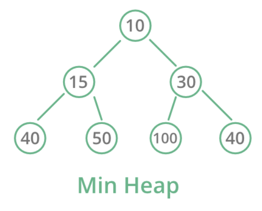
The root is 10 (smallest). Each parent is ≤ its children. Notice that the heap doesn’t fully sort — siblings can be in any order, and a value in one subtree can be less than values in another subtree, as long as the parent-child invariant holds locally.

Max-heap

Same idea, opposite direction:

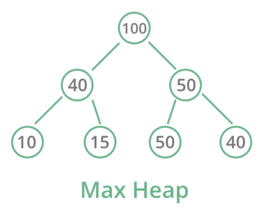
Root is the largest; each parent is ≥ its children.

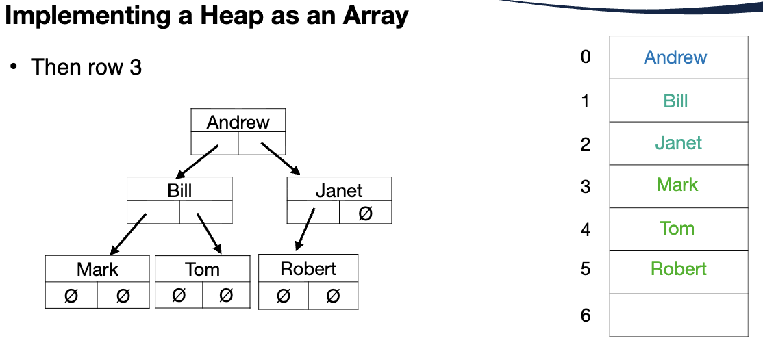
Heap as array

Because a heap is a complete binary tree, it can be stored efficiently in an array — no node pointers needed. The mapping:

For a node at index $i$:

$\text{leftChild}(i)=2i+1$

$\text{rightChild}(i)=2i+2$

$\text{parent}(i)=\lfloor (i-1)/2\rfloor$

So the root is at index 0, its children at 1 and 2, their children at 3, 4, 5, 6, and so on level by level.

This array representation saves memory (no pointers) and gives excellent cache locality. The trade-off: the array has a fixed capacity, and growing past it requires reallocating to a larger array and copying every element ($O(n)$ on the resizing operation, amortized $O(1)$ if you double the capacity each time). A pointer-based heap can grow one node at a time but pays cache and pointer overhead per node.

Example: in the array [Andrew, Bill, Janet, Mark, Tom, Robert]:

• Andrew is at 0 (root).
• Bill (1) and Janet (2) are children of Andrew.
• Mark (3) and Tom (4) are children of Bill.
• Robert (5) is the (only) child of Janet.

To find Robert’s parent: $(5-1)/2=2$ → Janet. ✓

Insert

To add a value:

1. Append the value at the end of the array (next open slot, position length).
2. Compare with parent. If the heap property is violated (e.g., new value < parent in a min-heap), swap.
3. Repeat with the new position until the heap property holds (or we’re at the root).

This is called sift up (or bubble up).

Cost: O(log n) — at most as many comparisons as the tree’s height.

Extract (remove root)

To remove the root:

1. Save the root value (this is what extract returns).
2. Move the last element (highest array index) into the root position.
3. Decrement the array’s used length.
4. Sift down the new root: compare with its children. If the heap property is violated, swap with the smaller (for min-heap) or larger (for max-heap) child. Repeat at the new position until done.

Worked example. Min-heap stored as [3, 5, 8, 9, 10, 12, 15]:

        3
      /   \
     5     8
    / \   / \
   9  10 12 15

Extract the root (3):

1. Save 3 as the return value.
2. Move the last element (15) to the root: [15, 5, 8, 9, 10, 12].
3. Sift down. Children of 15 are 5 (left) and 8 (right). The smaller child is 5, and 5 < 15, so swap: [5, 15, 8, 9, 10, 12].
4. 15 is now at index 1. Its children are 9 (index 3) and 10 (index 4). Smaller is 9, and 9 < 15, so swap: [5, 9, 8, 15, 10, 12].
5. 15 is now at index 3. Index 3 has no children (we’d need indices 7 and 8, beyond the array). Stop.

Final heap: [5, 9, 8, 15, 10, 12] — the heap property is restored, and 3 was returned.

Cost: O(log n) — at most one swap per level, traversing the tree’s height.

Build heap from an unsorted array

Given an array of $n$ values, you can turn it into a heap in place in $O(n)$ time. The trick is to sift-down each non-leaf node starting from the last one and walking back to the root:

buildHeap(A):
  for i = floor(n/2) - 1 down to 0:
    siftDown(A, i, n)

The leaf nodes (indices $\lfloor n/2\rfloor$ through $n-1$) are already trivially heaps of size 1. We only need to fix the internal nodes.

Why it’s O(n), not O(n log n)

The naive bound is ”$n$ sift-downs, each $O(\log n)$, so $O(n\log n)$.” That’s an overcount. Most nodes are near the bottom and have very short sift paths.

For a heap of $n$ nodes (a complete binary tree of height $h=\lfloor {\log }_{2}n\rfloor$):

• Level $h$ (leaves): about $n/2$ nodes, each with sift-down cost 0.
• Level $h-1$: about $n/4$ nodes, sift-down cost at most 1.
• Level $h-2$: about $n/8$ nodes, sift-down cost at most 2.
• …
• Level 0 (root): 1 node, sift-down cost at most $h$.

A node at height $j$ from the bottom has at most $\lceil n/2^{j+1}\rceil$ such nodes, each with sift-down cost at most $j$. Total work:

$T(n)\le {\sum }_{j=0}^h\frac{n}{2^{j+1}}\cdot j=\frac{n}{2}{\sum }_{j=0}^h\frac{j}{2^j}$

The sum ${\sum }_{j=0}^{\infty }j/2^j$ converges to 2 (standard result for $\sum j{x}^j=x/(1-x{)}^2$ at $x=1/2$). So

$T(n)\le \frac{n}{2}\cdot 2=n=O(n)$

The intuition: most of the nodes (the bottom half) sit at sift-paths of length 0 or 1, which dominate the count. The few nodes that pay $O(\log n)$ sift cost are at the top, and there are very few of them.

Stability

Heap-based sorting (like Heap sort) is not stable — equal elements can change relative order during swaps. If FIFO order matters for equal-priority items, you need to augment the priority with a tiebreaker (insertion order, time stamp, etc.).

The Canadian Triage and Acuity Scale is a real-world example: medical priority levels 1–5 (Resuscitation, Emergent, Urgent, Less Urgent, Non-Urgent) — patients within the same level should be served first-come-first-served, but a plain max-heap might shuffle them.

Why heaps work in O(log n)

A heap is a complete binary tree, so its height is exactly $\lfloor {\log }_{2}n\rfloor$. Both insert (sift up) and extract (sift down) traverse at most this height, giving $O(\log n)$ per operation.

The completeness is what makes the array representation work — every position is filled in level order, so we never have “gaps” in the array.

Use cases

• Priority queues — process scheduling, event simulation, network packet prioritization.
• Heap sort — sort an array using a heap. See Heap sort.
• Dijkstra’s algorithm — efficient extraction of the next vertex by shortest distance. See Dijkstra’s algorithm.
• Top-K selection — keep a heap of size K to track the K largest/smallest items in a stream.

For the heap-based sorting algorithm specifically, see Heap sort. For the more general priority queue concept, the heap is the standard implementation.