A heat map uses color to represent the value at each cell of a two-dimensional grid. It’s the natural way to visualize a matrix: anything where we have a value indexed by two categorical or two binned-numerical dimensions.
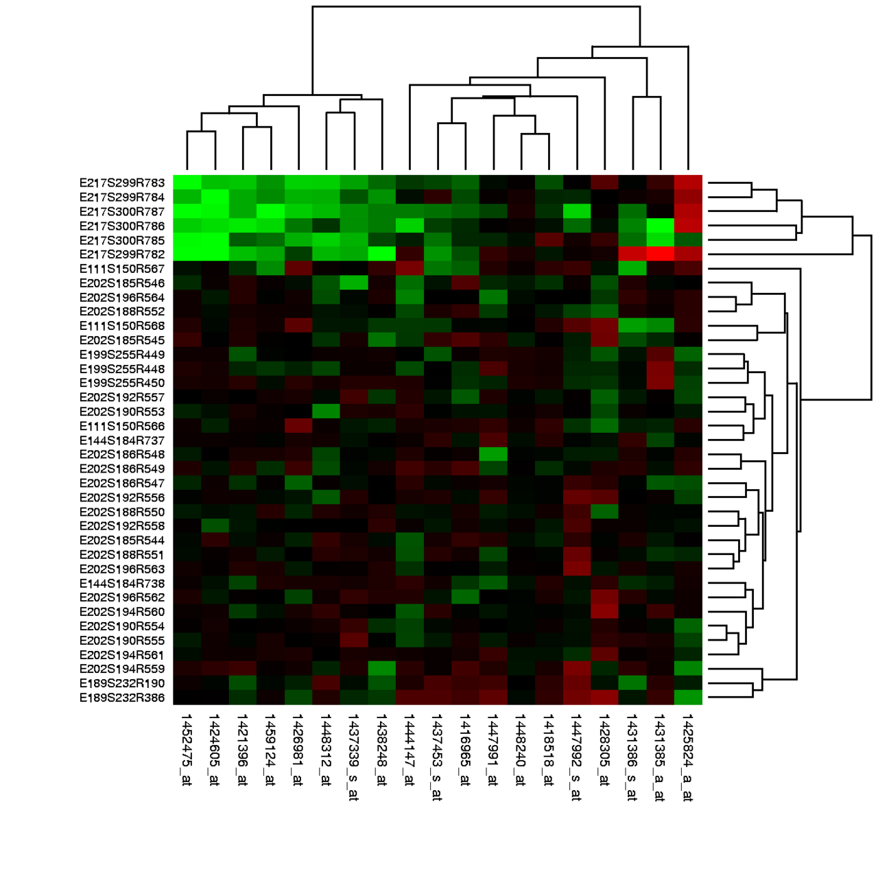 Image: Heat map of DNA microarray expression data, public domain
The classic example in machine learning is the Confusion matrix: rows are true classes, columns are predicted classes, and the color of cell shows how often class was predicted as class . A perfect classifier produces a heat map with bright cells on the diagonal and dark cells everywhere else; a confused classifier shows off-diagonal brightness wherever it makes systematic mistakes.
Other common uses:
- Correlation matrices: a square heat map where cell shows the correlation between feature and feature . The diagonal is always 1; off-diagonal patterns reveal which features move together.
- Geographic data on a regular grid: temperature, rainfall, population density. Each cell is a geographic patch, color shows the value.
- Genomic data: gene expression across samples, where rows are genes, columns are conditions, color is expression level.
- Time-by-category visualizations: number of customers by hour and day of week, energy usage by month and year.
The choice of colormap matters. Sequential colormaps (viridis, plasma, magma) work for values that have a natural ordering low-to-high. Diverging colormaps (red-white-blue, say) work when the meaningful axis is distance from a neutral midpoint: positive vs. negative correlations, deviations above and below a baseline. Qualitative colormaps (tab10, Pastel1) are the wrong choice for heat maps because their colors aren’t ordered.
In Matplotlib, ax.imshow(matrix, cmap='viridis') draws a heat map. plt.colorbar(...) adds the legend that maps colors back to numeric values. Without a colorbar a heat map is impossible to read precisely.