t-SNE (t-distributed stochastic neighbor embedding) is a non-linear Dimensionality reduction method. Where PCA looks for directions of maximum variance (a linear projection), t-SNE looks for low-dimensional positions that preserve neighborhood structure from the high-dimensional space.
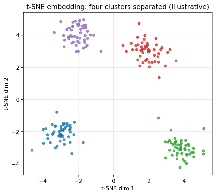 Idealised t-SNE embedding: four high-dimensional clusters mapped to 2-D with distinct neighbourhoods preserved.
The intuition: instead of asking which directions have the most variance, t-SNE asks which points are close to which other points, then arranges the points in low-dimensional space so that close pairs stay close and distant pairs stay distant.
More precisely:
- In the original high-dimensional space, define a probability distribution over pairs of points: close pairs get high probability, distant pairs get low probability.
- In the low-dimensional embedding (typically 2D), define a similar probability distribution using a Student’s -distribution (the t in t-SNE).
- Adjust the low-dimensional positions to make the two distributions match as closely as possible.
The visual consequence is that clusters that exist in the original data tend to appear as visually distinct clusters in the projection. Two points close in 10-dimensional space stay close in the 2D plot; two points far apart stay far apart. The result is a scatter plot where clusters jump out.
The mathematical details (the specific form of the probability distributions, the optimization procedure that adjusts positions) are out of scope for the Introduction to Data Science course. More mathematical details require advanced statistics and optimization algorithms, the textbook says, and leaves it at that.
In scikit-learn, t-SNE is in sklearn.manifold:
from sklearn.manifold import TSNE
tsne = TSNE(n_components=2, perplexity=30, learning_rate='auto', init='pca')
X_tsne = tsne.fit_transform(X_original)n_components=2requests a 2D embedding.perplexity=30is roughly the effective number of neighbors t-SNE considers when building its probability distributions. 30 is a typical default.learning_rate='auto'andinit='pca'are the recommended defaults.
Comparing PCA and t-SNE. Running both on the same dataset is worth doing. PCA gives an elliptical cloud with the classes interspersed throughout; t-SNE gives a clustered structure with local patches. Neither is correct, they show different aspects of the same data. PCA preserves global linear structure; t-SNE preserves local neighborhood structure.
A reproducibility caveat. With init='random', t-SNE’s result depends on the random initialization, and two runs on the same data can produce visually different plots: different rotations, different cluster placements. init='pca' (the recommended default in modern scikit-learn) is much more reproducible because it starts from a deterministic PCA projection. Setting random_state fixes the seed for full reproducibility.
What t-SNE plots don’t tell you
t-SNE is a visualization tool and should be read like one: patterns suggest hypotheses, they don’t prove them. A few things beginners over-read:
- Distances in the embedding are not meaningful. Two points that look 1 unit apart aren’t “twice as similar” as points 2 units apart. The embedding only tries to preserve a local ordering of neighbors, not metric distances. Global geometry, the gaps between clusters and the overall layout, is arbitrary.
- Cluster sizes are not meaningful. A tight cluster in the plot isn’t a tighter cluster in the original data. t-SNE’s choice of how dense to draw each cluster depends on the local density of neighbors and the perplexity setting, not on the data’s actual variance.
- t-SNE can create spurious clusters. With certain perplexity settings, especially low ones, t-SNE can fracture a single continuous distribution into apparent clusters that don’t exist in the original space. Running with multiple perplexities (5, 30, 50) and looking for cluster structure that’s stable across settings is the standard mitigation.
- No inverse transform / no new-data projection. t-SNE is fit to a specific dataset; there’s no
transform()method that maps a new point into the existing embedding. Adding new data requires refitting from scratch, at which point even the original points may end up in different positions. PCA, UMAP, and autoencoders all support out-of-sample projection; t-SNE does not. This is a hard limitation, not an oversight.
If clusters in a t-SNE plot are interesting, the right next step is to verify them — either with a clustering algorithm run on the original high-dimensional data, or by checking class labels (if available) for separability in the original space.
t-SNE was introduced by Laurens van der Maaten and Geoffrey Hinton in 2008 as an improvement over the earlier SNE (stochastic neighbor embedding), specifically by switching the low-dimensional similarity from a Gaussian to a Student’s -distribution. The heavier tails of the better accommodate the geometry of low-dimensional space and reduce the “crowding problem.”