Existence and uniqueness theorem

Two questions about an Initial value problem: does a solution exist, and is it the only one?

For the IVP $y^{\prime }=f(x,y)$, $y(x_0)=y_0$:

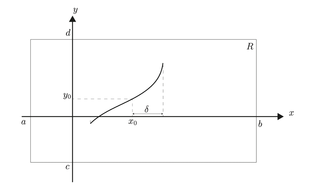
If $f$ and $\frac{\partial f}{\partial y}$ are continuous in some rectangle $R=\{(x,y):a<x<b,c<y<d\}$ containing $(x_0,y_0)$, then the IVP admits a unique solution $\varphi$ defined on some interval $(x_0-\delta ,x_0+\delta )$ for some $\delta >0$.

This is a textbook simplification of two separate theorems:

• Peano existence theorem: continuity of $f$ alone is enough to guarantee that at least one solution exists locally. No uniqueness.
• Picard–Lindelöf theorem: $f$ continuous and Lipschitz continuous in $y$ guarantees existence and uniqueness. The standard textbook hypothesis ”$\partial f/\partial y$ continuous” is a strictly stronger condition that implies Lipschitz on any compact set, which is why it’s used in introductory courses: easier to verify, slightly weaker than necessary.

So in practice:

• Continuity of $f$ alone $\Rightarrow$ at least one solution exists (Peano).
• Continuity of $f$ and Lipschitz in $y$ (e.g., $\partial f/\partial y$ continuous) $\Rightarrow$ that solution is unique (Picard–Lindelöf).

The solution is local, guaranteed only in a small interval around $x_0$, not globally.

Intuition

Think of $f(x,y)$ as a slope field: it tells you the slope of any solution curve at every point $(x,y)$.

If $f$ is continuous, the slope field has no gaps. You can follow the slope arrows starting at any point and trace out a smooth curve. So a solution exists.

If $\frac{\partial f}{\partial y}$ is also continuous, nearby slopes don’t change too abruptly — two solution curves can’t merge or branch off each other. So the solution is unique: only one path through any given point.

The rectangle $R$ is the “safe zone” where $f$ behaves nicely. The number $\delta$ measures how far you can move horizontally from $x_0$ while staying inside the safe zone.

Why both conditions matter

Continuity of $f$ is sufficient for existence (Peano’s theorem). Without it the slope field can have a “hole” and no smooth path through. Continuity isn’t strictly necessary. Some discontinuous $f$ still admit solutions (e.g. $y^{\prime }=\mathrm{sgn}(x)$, $y(0)=0$ has solution $y=|x|$), but with continuity you’re guaranteed at least one.

Continuity of $\frac{\partial f}{\partial y}$ (or, more generally, $f$ being Lipschitz in $y$) is sufficient for uniqueness. Without it, two solutions can pass through the same point.

Worked example of failure: $y^{\prime }=\frac{y}{x}$ at $(0,0)$.

$f(x,y)=y/x$ is undefined at $x=0$, so the rectangle around $(0,0)$ contains points where $f$ isn’t defined.

The IVP $y^{\prime }=y/x$, $y(0)=0$ has solutions $y=cx$ for every $c$. Infinitely many solutions through $(0,0)$.

Worked example of existence failure: $y^{\prime }=y/x$, $y(0)=1$. At $x=0$, $y/x\to \infty /0$ undefined. No solution at $x=0$.

Worked example: showing the theorem applies

The IVP $y^{\prime }=3x+\sin y$, $y(0)=1$.

$f(x,y)=3x+\sin y$ is continuous everywhere on ${\mathbb{R}}^2$. Its partial derivative $\frac{\partial f}{\partial y}=\cos y$ is also continuous everywhere.

At $(0,1)$, both are continuous. So the theorem guarantees a unique local solution $\varphi$ defined on some interval $(0-\delta ,0+\delta )$ around $x=0$.

The theorem doesn’t say what $\delta$ is, or how to find $\varphi$. It just guarantees existence and uniqueness.

Linear ODEs: stronger result

For first-order linear ODEs in standard form $y^{\prime }+P(x)y=Q(x)$, a stronger result holds: if $P$ and $Q$ are continuous on an open interval $I$ containing $x_0$, then the IVP has a unique solution defined on all of $I$, globally, not just locally.

This is because linear ODEs can be explicitly solved via the Integrating factor method, and the solution formula is well-defined as long as the integrating factor and the integrals exist.

What it doesn’t say

Three things the theorem doesn’t tell you:

1. The size of $\delta$. Just that some $\delta >0$ works.
2. How to find the solution. The theorem is non-constructive.
3. What happens if conditions fail. Failure of continuity doesn’t mean no solution exists, only that the theorem doesn’t guarantee anything.

For a constructive way to build the solution the theorem promises, see Picard iteration.