Gradient descent

Gradient descent is an iterative optimization algorithm that minimizes a function by repeatedly stepping in the direction of the negative Gradient. It’s the standard tool for training virtually all modern machine-learning models, from Linear regression through deep neural networks.

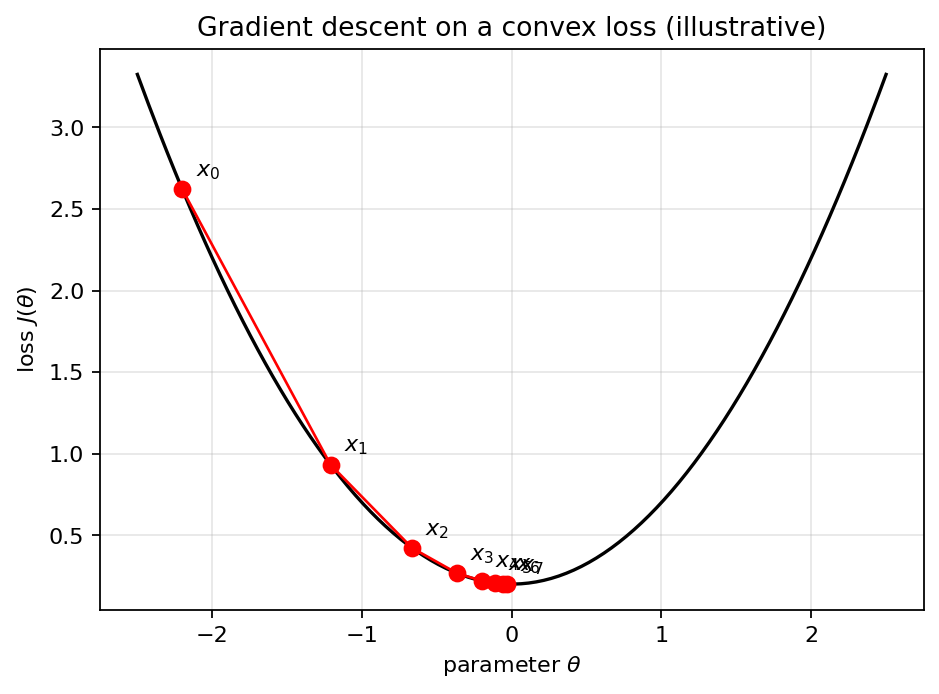
The picture: imagine a hilly landscape where the elevation at each point represents the loss for the corresponding parameter values. We’re standing somewhere on the landscape — at some current $\mathbf{w}$ — and we want to find the lowest point. We can’t see the whole landscape; we can only feel the slope under our feet. The natural strategy is to take small steps downhill. As long as we’re going downhill, we’re getting closer to a minimum.

The update rule

The mathematics that formalizes downhill is the Gradient. The negative gradient $-\nabla J$ points in the direction of steepest decrease. The update rule:

${\mathbf{w}}_{t+1}={\mathbf{w}}_t-\eta \nabla J({\mathbf{w}}_t)$

At step $t$, evaluate the gradient at the current parameters ${\mathbf{w}}_t$, multiply by the Learning rate $\eta$, and subtract. Repeat.

If $\eta$ is too small, training is very slow — we creep down the hill in tiny steps. If $\eta$ is too large, the updates may overshoot the minimum and the loss may oscillate or even increase. A good learning rate lets the model move steadily toward the minimum at a reasonable pace.

Why iterative

For Linear regression with Mean squared error, the minimum has a closed-form solution: take partial derivatives, set them to zero, solve. Direct computation, no iteration.

For more complex models — neural networks, deep architectures with millions of parameters — the closed form breaks down. Solving the equations becomes intractable. Iterative methods like gradient descent are the only practical approach.

Even when a closed form exists, gradient descent is sometimes preferred because it scales better to huge datasets (using stochastic or minibatch variants that update on a subset of the data per step rather than the entire training set).

Variants

Batch gradient descent uses the full training set to compute the gradient at each step. Accurate gradient estimates, slow on big datasets.

Stochastic gradient descent (SGD) uses one example per step. Noisy gradient estimates, much faster, often produces good final results because the noise helps escape bad local minima.

Minibatch gradient descent uses a small subset (say 32 or 128 examples) per step. The middle ground — reasonably accurate gradients, fast updates. This is what most modern ML training actually uses.

Adaptive methods (Adam, RMSProp, AdaGrad) adjust the learning rate per parameter based on the history of gradients. Often converge faster than plain gradient descent and are less sensitive to the initial learning rate.

Convergence

For convex losses (like Mean squared error for linear regression, or Binary cross-entropy for Logistic regression without regularization peculiarities) gradient descent provably converges to the global minimum given a small enough learning rate — every local minimum of a convex function is global. For non-convex losses (typical of deep neural networks), it converges to a local minimum, not necessarily the best one. Saddle points slow training but stochastic-gradient noise typically escapes them. In practice, for large neural networks, the many local minima tend to have similar loss values, so finding “a” local minimum is usually fine — but the convergence guarantee from the convex case is gone.

This procedure — initialize parameters, compute predictions, compute loss, compute gradients, step — is the engine driving virtually all modern machine-learning training. Every neural network, no matter how large, is trained by some variant of this loop.