Logistic regression

Logistic regression is a binary classification model that applies the Sigmoid function to a linear combination of inputs to produce a probability of class 1. Despite the name, it’s a classifier, not a regressor. The regression refers to the linear function inside, but the output is a discrete class.

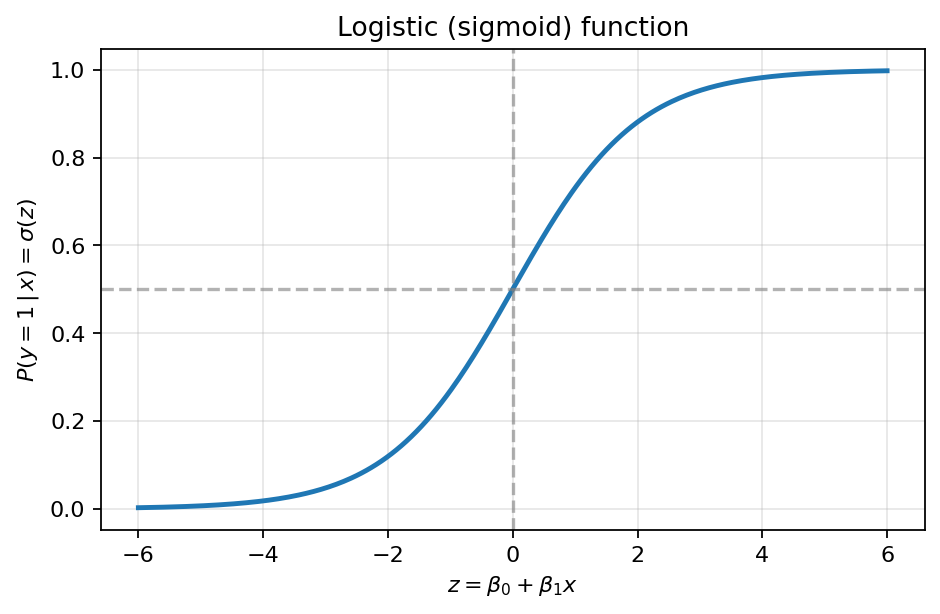Sigmoid function mapping a linear predictor $z={\beta }_0+{\beta }_{1}x$ to a probability in $(0,1)$.

The model

Define a linear function of the inputs:

$z=w_0+w_1{x}_1+w_2{x}_2+\cdots +w_m{x}_m$

This is the same expression used in Linear regression. It can take any real value. Wrap it in the sigmoid:

$\hat{p}(y=1\mid \mathbf{x})=\frac{1}{1+e^{-z}}$

The notation $\hat{p}(y=1\mid \mathbf{x})$ reads as the predicted probability that the class is 1, given the input $\mathbf{x}$. The hat means predicted by the model; the bar means given that. The output is bounded between 0 and 1 by the sigmoid, and makes sense as a probability.

To turn this into a hard classification, threshold at 0.5:

$\hat{y}=\{\begin{array}{ll}1& \text{if }\hat{p}(y=1\mid \mathbf{x})\ge 0.5\\ 0& \text{otherwise}\end{array}$

The decision boundary is the surface where $\hat{p}=0.5$, equivalently where $z=0$. For two input features, this is a straight line in feature space; for three, a plane; in general, a hyperplane.

Training

Logistic regression is trained with Gradient descent using Binary cross-entropy as the Loss function:

$J(\mathbf{w})=-\frac{1}{N}{\sum }_{i=1}^N\left[y_i\log f(x_i)+(1-y_i)\log (1-f(x_i))\right]$

The $1/N$ averages over the dataset; some textbooks drop it and use the un-normalized sum, which doesn’t change the minimizer. The cross-entropy loss penalizes confident mistakes much more harshly than uncertain ones. We can’t use Mean squared error here — MSE combined with the sigmoid produces a non-convex loss surface, so gradient descent has weaker guarantees and can stall in flat regions. Cross-entropy with sigmoid gives a clean convex bowl that gradient descent reliably finds the bottom of.

The training loop is the standard one:

1. Initialize parameters $\mathbf{w}$.
2. Compute predictions $f(x_i)$ for every training example.
3. Compute the loss.
4. Compute the gradient $\nabla J(\mathbf{w})$.
5. Update: $\mathbf{w}\leftarrow \mathbf{w}-\eta \nabla J(\mathbf{w})$.
6. Repeat until convergence.

In scikit-learn

from sklearn.linear_model import LogisticRegression
from sklearn.pipeline import make_pipeline
from sklearn.preprocessing import StandardScaler
 
clf = make_pipeline(StandardScaler(), LogisticRegression(max_iter=10000))
clf.fit(X_train, y_train)
y_pred = clf.predict(X_test)
y_prob = clf.predict_proba(X_test)

predict() returns the hard class label (0 or 1). predict_proba() returns an $N\times 2$ array where the first column is the probability of class 0 and the second is the probability of class 1. Each row sums to 1. The second column is what we use to compute the ROC curve and AUC.

max_iter=10000 controls the maximum number of optimizer iterations. The default 100 is sometimes too few for the optimizer to converge on real datasets; 10000 is a generous upper bound.

The make_pipeline(StandardScaler(), LogisticRegression(...)) pattern is the standard way to avoid Data leakage. The StandardScaler is fit only on training data and the same fitted scaling is applied to test data.

Limitations

Logistic regression is a linear classifier: its decision boundary is a hyperplane. It can’t capture non-linear class boundaries directly. The standard workarounds are:

• Feature engineering: hand-craft non-linear features (squared, interaction, log-transformed) so the boundary in the engineered feature space is linear.
• Kernel methods: implicitly map inputs to a higher-dimensional space where the boundary is linear.
• Neural networks: stack many logistic regressions, learning a non-linear decision boundary end-to-end.

For the canonical wine-quality and heart-disease examples in the Introduction to Data Science textbook, logistic regression gets to roughly 73-80% accuracy with AUC around 0.80. Respectable, well above random, but limited by the linearity assumption.