Phase plane

The phase plane is the 2D plot of $(x,y)$ for a system ${\mathbf{x}}^{\prime }=\mathbf{F}(\mathbf{x})$ in ${\mathbb{R}}^2$. Instead of plotting $x(t)$ and $y(t)$ separately as functions of time, you plot the trajectory $(x(t),y(t))$ as a curve traced through the plane.

For a 2D autonomous system, the trajectory’s shape (geometry) doesn’t depend on how fast it’s traversed, only on the relationship between $x$ and $y$. This is why phase-plane analysis decouples geometry from time and gives qualitative insight into the system’s long-term behavior.

The generalization to higher dimensions is phase space, but it’s much harder to visualize.

The phase plane equation

For a 2D autonomous system

$\{\begin{array}{l}{x}^{\prime }=f(x,y)\\ y^{\prime }=g(x,y)\end{array}$

eliminate $t$ via the chain rule:

$\frac{dy}{dx}=\frac{dy/dt}{dx/dt}=\frac{g(x,y)}{f(x,y)}$

This is the phase plane equation. It relates $y$ and $x$ directly without time. Solving it (when possible) gives the trajectories.

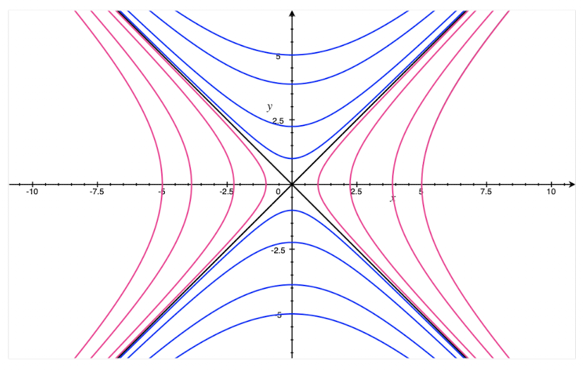
For example, $\{\begin{array}{l}{x}^{\prime }=y\\ y^{\prime }=x\end{array}$ gives phase plane equation $\frac{dy}{dx}=x/y$. Separable: $ydy=xdx$, integrate: $y^2-x^2=c$. Trajectories are hyperbolas.

When the phase plane equation is hard

For most nonlinear systems, the phase plane equation $dy/dx=g/f$ can’t be solved in closed form. But you can still:

• Find equilibria: solve $f=0$ and $g=0$ simultaneously.
• Compute the slope field: at each $(x,y)$, the trajectory has slope $g/f$. Plot the direction at a grid of points.
• Numerically integrate to trace specific trajectories.
• Linearize around equilibria (see Locally linear system) to find local behavior.
• Apply Lyapunov’s method for stability without explicit solutions.

Why the phase plane matters

Long-term behavior of a 2D system is determined by:

1. Where the equilibria are.
2. What kind of equilibrium each is (stable node, saddle, spiral, etc.).
3. How trajectories connect them (or escape to infinity).

The phase plane visualizes all this. A glance at the phase portrait tells you whether the system oscillates, converges, diverges, or has multiple stable basins.

Standard equilibrium types in the linear case: Phase plane behaviour. Formal stability theory: Stability of autonomous systems.

Phase plane vs slope field

Closely related:

• Slope field (or direction field): at each point $(x,y)$, draw a small arrow with slope $g/f$. Doesn’t show specific trajectories, just the direction of flow at each point.
• Phase portrait: actual trajectory curves through the plane.

A slope field is a “vector field” view; a phase portrait is the “integral curves” view. The slope field is easier to compute (just evaluate $g/f$ everywhere); the phase portrait is more informative (shows actual flow paths). Tools like Wolfram Alpha or Matlab plot both side by side.

Examples in nature

• Pendulum in phase plane $(\theta ,\dot{\theta })$: closed orbits around the rest position (stable center), separatrices through the inverted position (saddle).
• Predator-prey: closed orbits indicating periodic population cycles.
• Damped oscillator: spiral inward to origin (asymptotically stable spiral).
• Limit cycles (in some nonlinear systems): isolated closed orbits that nearby trajectories spiral toward. Explains self-sustained oscillations like heartbeat.

See Autonomous system.