Phase plane behaviour

For a 2D linear autonomous system ${\mathbf{x}}^{\prime }=A\mathbf{x}$, the phase portrait (qualitative picture of trajectories in the $xy$-plane) is set by the eigenvalues of $A$. Six standard cases cover everything, each with its own shape and stability.

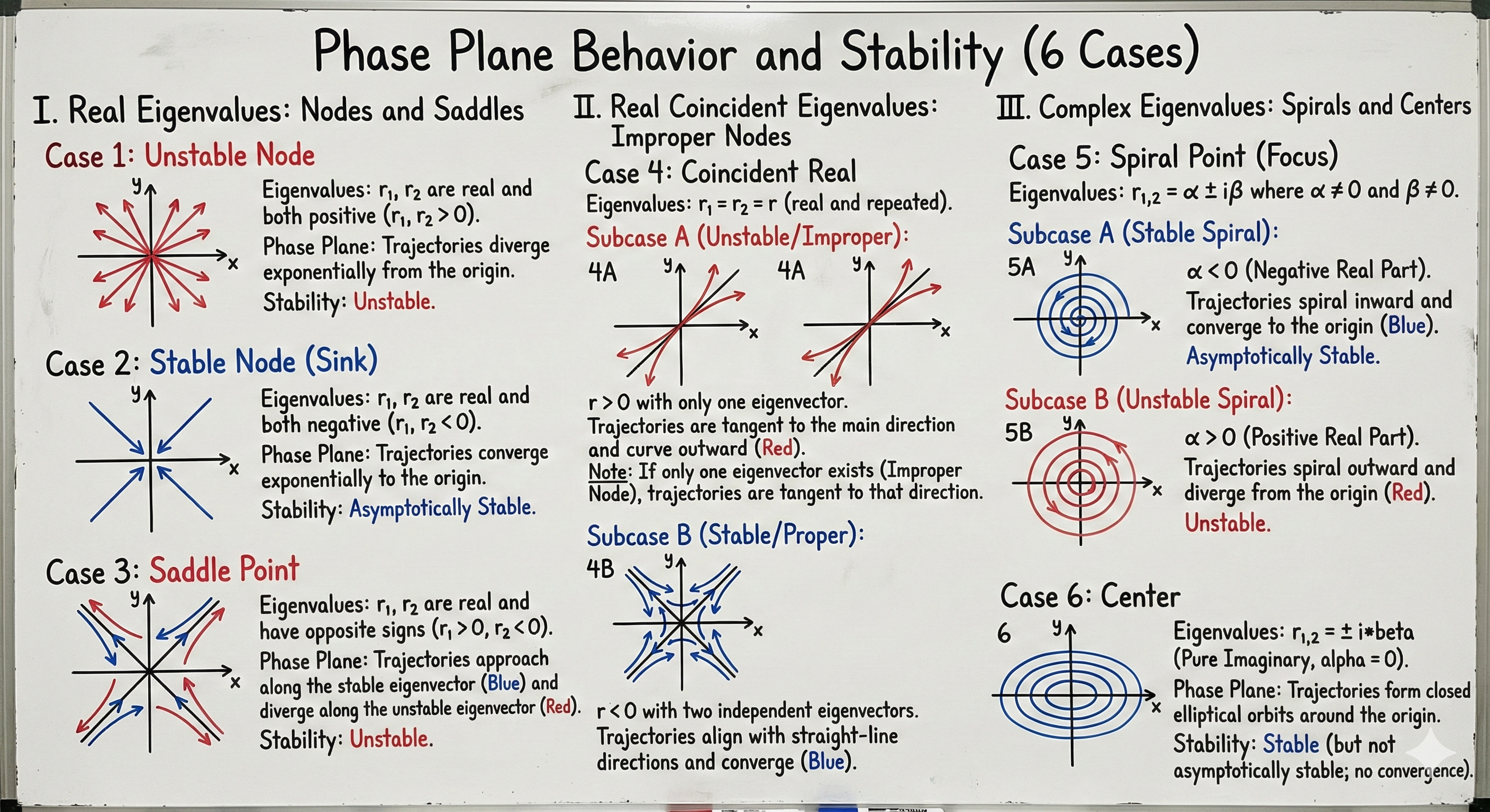All six cases on a single whiteboard: Case 1 unstable node, Case 2 stable node (sink), Case 3 saddle, Case 4 repeated-eigenvalue nodes (proper/improper), Case 5 spirals, Case 6 center.

Stability terminology

Quick recap (formal definitions in Stability of autonomous systems):

• Stable: nearby trajectories stay nearby for all time.
• Asymptotically stable: nearby trajectories converge to the equilibrium.
• Unstable: at least some nearby trajectories move away.

Phase portrait classifications:

• Node: trajectories approach (or leave) along straight-line directions.
• Saddle: trajectories approach along one direction, depart along another.
• Spiral (focus): trajectories spiral in or out.
• Center: trajectories form closed orbits.

Case 1: distinct real eigenvalues, both positive ($r_1\ne r_2>0$)

Both eigenvalues positive real. Solutions $\mathbf{x}(t)=c_1{\mathbf{u}}_1{e}^{r_{1}t}+c_2{\mathbf{u}}_2{e}^{r_{2}t}$ grow exponentially in both eigenvector directions.

• Type: unstable node. (Some introductory texts call this an “improper node,” but in standard dynamical-systems terminology “improper” denotes the defective repeated-eigenvalue case in Case 4b below; with two distinct eigenvalues this is just a node.)
• Behavior: trajectories diverge exponentially from the origin.
• Equilibrium stability: unstable.

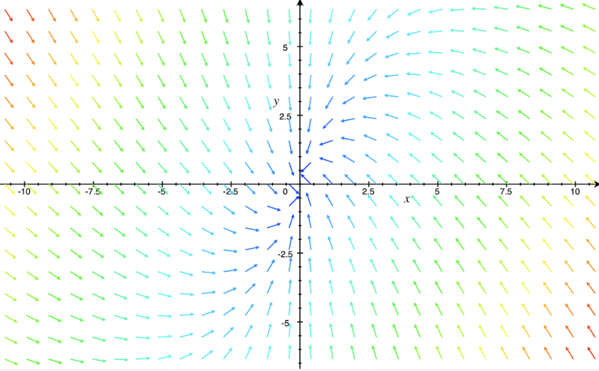
Case 2: distinct real eigenvalues, both negative ($r_1\ne r_2<0$)

Both eigenvalues negative real. Mirror of Case 1: trajectories shrink toward origin.

• Type: stable node (sink).
• Behavior: trajectories converge exponentially to origin.
• Equilibrium stability: asymptotically stable.

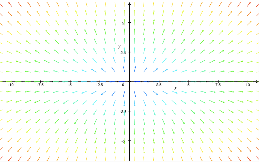
Case 3: distinct real eigenvalues, opposite signs ($r_1>0>r_2$)

One positive, one negative. Solutions grow in one direction, shrink in another.

• Type: saddle point.
• Behavior: trajectories approach origin along the eigenvector for the negative eigenvalue, then diverge along the positive eigenvalue’s direction.
• Equilibrium stability: unstable.

Case 4: repeated real eigenvalues ($r_1=r_2=r$)

Two subcases depending on number of eigenvectors:

Case 4a: two linearly independent eigenvectors (proper node)

Every direction is an eigenvector: the matrix is a scalar multiple of identity. Trajectories are straight lines through origin.

• $r>0$: unstable proper node.
• $r<0$: stable proper node (asymptotically stable).

Case 4b: only one eigenvector (improper node)

Defective matrix (the Repeated eigenvalues case). Trajectories curve, tangent to the eigenvector direction near origin.

• $r>0$: unstable improper node.
• $r<0$: stable improper node (asymptotically stable).

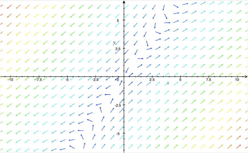
Case 5: complex conjugate eigenvalues with nonzero real part ($r=\alpha \pm i\beta$, $\alpha \ne 0$)

The system has oscillatory behavior with exponential envelope.

In polar coordinates $(\rho ,\theta )$, the radius evolves as $\rho (t)={\rho }_0{e}^{\alpha t}$, so exponential growth or decay. The angle changes at rate $\beta$.

• $\alpha >0$: trajectories spiral outward. Unstable spiral.
• $\alpha <0$: trajectories spiral inward to origin. Asymptotically stable spiral.

The direction of rotation depends on the sign of $\beta$.

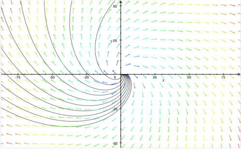
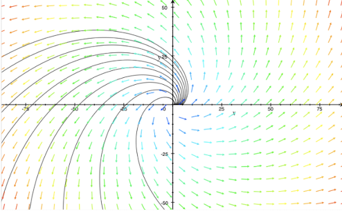
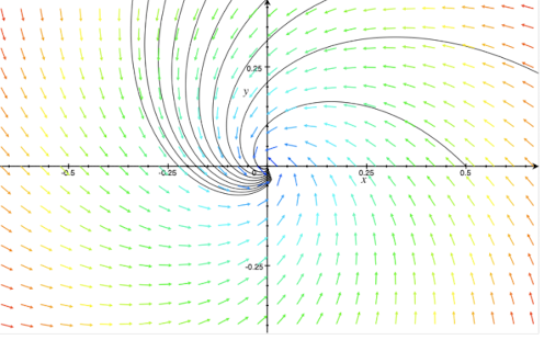
The four spiral images show: $\alpha >0,\beta >0$ (unstable counterclockwise); $\alpha >0,\beta <0$ (unstable clockwise); $\alpha <0,\beta <0$ (stable clockwise); $\alpha <0,\beta >0$ (stable counterclockwise).

Case 6: pure imaginary eigenvalues ($r=\pm i\beta$, $\beta \ne 0$)

No exponential envelope ($\alpha =0$). Trajectories are closed orbits (ellipses around the origin), with period $T=2\pi /\beta$.

• Type: center.
• Behavior: bounded periodic motion forever.
• Equilibrium stability: stable but not asymptotically stable.

Summary table

Eigenvalues	Type	Stability
Real distinct, both $>0$	Node	Unstable
Real distinct, both $<0$	Node (sink)	Asymptotically stable
Real distinct, opposite signs	Saddle	Unstable
Real repeated, 2 eigenvectors	Proper node	Stable iff $r<0$
Real repeated, 1 eigenvector	Improper node	Stable iff $r<0$
Complex, $\alpha >0$	Spiral	Unstable
Complex, $\alpha <0$	Spiral	Asymptotically stable
Pure imaginary	Center	Stable, not asymptotically

Why this classification matters

For 2D linear autonomous systems, the eigenvalues of $A$ tell you everything about long-term behavior, no need to solve the ODE. Each phase portrait shape goes with a different qualitative behavior, and the eigenvalues alone pick which one.

It also carries over to nonlinear systems. By the linearization theorem, near any equilibrium of a nonlinear system the local phase portrait resembles one of these six cases (when the eigenvalues are off the imaginary axis). See Locally linear system for that technique.