Level-order traversal

Level-order traversal visits the nodes of a Binary tree in order of depth: first the root (depth 0), then all depth-1 nodes (root’s children), then all depth-2, and so on. Within a level, traverse left to right.

This is the binary-tree case of BFS: it explores nodes layer by layer rather than going deep first. The other three traversals (pre-, in-, post-order) are depth-first; level-order is breadth-first, structurally different.

Why a queue, not a stack

The depth-first orders use a stack (explicit or recursive call stack) because each “go deeper” call holds the parent’s state until the deeper call returns. That’s LIFO behaviour — the last unfinished caller is the first to resume.

Level-order is FIFO: nodes discovered earlier (closer to the root) must be processed earlier than nodes discovered later (deeper). A Queue gives exactly that — first in, first out.

So level-order doesn’t recurse naturally — it needs an explicit queue.

Implementation

void levelOrderTraversal(BinaryTreeNode *node) {
    if (node == NULL) return;
    Queue q = queue_create();
    enqueue(&q, node);
    while (!queue_empty(&q)) {
        BinaryTreeNode *cur;
        dequeue(&q, &cur);
        printf("%d ", cur->data);
        if (cur->left  != NULL) enqueue(&q, cur->left);
        if (cur->right != NULL) enqueue(&q, cur->right);
    }
}

Algorithm:

Enqueue the root.
While the queue isn’t empty: dequeue a node, process it, enqueue its children left-to-right.

The queue invariant: at any moment, the queue holds a contiguous segment of nodes — the front of one level plus the back of the next. As you dequeue from the front, the level you’re processing shrinks; as you enqueue children, the next level grows.

Worked example

Take the standard sorted binary tree: root F; F’s children B (left) and G (right); B’s children A and D; D’s children C and E; G’s right child I, whose left child is H. Level-order sweeps the tree top-to-bottom, left-to-right within each row:

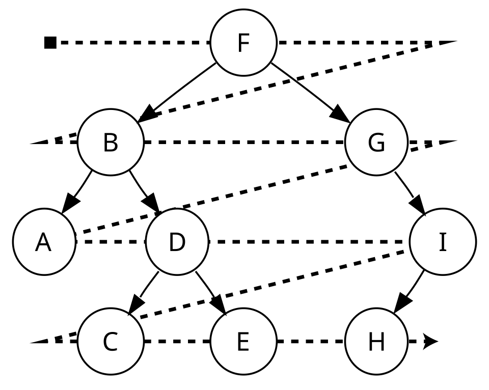Image: Sorted binary tree showing breadth-first (level-order) traversal, CC0 / public domain

Level-order output: F B G A D I C E H

Trace queue state (front on left):

Step	Queue	Action	Output
0	`[F]`	Initial
1	`[B, G]`	Dequeue F, enqueue B and G	`F`
2	`[G, A, D]`	Dequeue B, enqueue A and D	`F B`
3	`[A, D, I]`	Dequeue G, enqueue I (no left child)	`F B G`
4	`[D, I]`	Dequeue A, no children	`F B G A`
5	`[I, C, E]`	Dequeue D, enqueue C and E	`F B G A D`
6	`[C, E, H]`	Dequeue I, enqueue H (no right child)	`F B G A D I`
7	`[E, H]`	Dequeue C, no children	`F B G A D I C`
8	`[H]`	Dequeue E, no children	`F B G A D I C E`
9	`[]`	Dequeue H, no children	`F B G A D I C E H`

Notice the queue grows then shrinks: the breadth-first frontier swells as you reach wider levels and shrinks as you process them.

Distinguishing levels

The bare algorithm produces a flat sequence. To process one level at a time (e.g., print each level on its own line), record the queue’s size at the start of each level and consume exactly that many nodes:

void levelOrderByLevel(BinaryTreeNode *root) {
    if (root == NULL) return;
    Queue q = queue_create();
    enqueue(&q, root);
    while (!queue_empty(&q)) {
        int levelSize = queue_size(&q);
        for (int i = 0; i < levelSize; i++) {
            BinaryTreeNode *cur;
            dequeue(&q, &cur);
            printf("%d ", cur->data);
            if (cur->left)  enqueue(&q, cur->left);
            if (cur->right) enqueue(&q, cur->right);
        }
        printf("\n");
    }
}

The levelSize at iteration start equals the count of nodes at the current depth (everything at deeper levels gets enqueued during the loop and processed in the next outer iteration).

Use cases

Shortest path from root. In an unweighted graph (or tree), BFS finds the minimum-edge-count path. The depth at which you first encounter a node = shortest distance from the start.
Level-by-level processing. Print the tree by depth, find the maximum value at each depth, compute the average per level.
Tree width. The maximum number of nodes at any single depth = the queue’s maximum size during traversal.
Right view / left view of a tree. The first node at each level (left view) or the last (right view) — derived from the level-by-level form.
Serialisation that preserves depth. Useful when later reconstruction needs to know which nodes were on the same level.

Complexity

Time $O (n)$ — every node enqueued and dequeued once.

Space $O (w)$ where $w$ is the width of the widest level. For a complete binary tree with $n$ nodes, the bottom level holds about $n /2$ nodes, so worst-case queue space is $O (n)$ — worse than the depth-first orders’ $O (h) = O (lo g n)$ .

This is the trade-off: depth-first traversals use less space on balanced trees, breadth-first uses less on degenerate (long-skinny) trees. Pick based on the structure you expect.

Versus BFS on graphs

Level-order on a tree is BFS without the “visited set” — you don’t need to track visited nodes because trees have no cycles, so a child can never be reached twice. On a general Graph you do need a visited set; otherwise BFS loops forever on cycles. See Breadth-first search for the graph case.

Comparison

Order	Driver	Sequence	Space
Pre-order	Stack	Root, Left, Right	$O (h)$
In-order	Stack	Left, Root, Right	$O (h)$
Post-order	Stack	Left, Right, Root	$O (h)$
Level-order	Queue	By depth, left-to-right	$O (w)$

Stack-driven orders go deep; queue-driven order goes wide. For the hub note, see Binary tree traversal.

Idriss Rami — Notes

Explorer