Bode plot

A Bode plot is the standard graphical representation of an LTI system’s frequency response: two plots side-by-side or stacked, with the same logarithmic frequency axis.

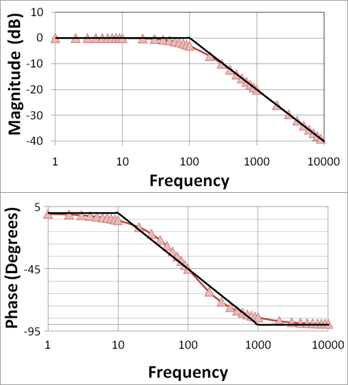Image: Bode magnitude and phase plots of a low-pass filter, CC0 / public domain — the straight-line asymptotic approximation (black) versus the actual response (red).

• Magnitude plot: $20{\log }_{10}|H(j\omega )|$ in decibels vs ${\log }_{10}(\omega )$.
• Phase plot: $\angle H(j\omega )$ in degrees (or radians) vs ${\log }_{10}(\omega )$.

The logarithmic frequency axis compresses a wide range (sometimes 6+ decades) into a readable picture, and the dB magnitude makes pole-zero structure visible at a glance.

Why logarithmic

Plotting $|H|$ on linear axes hides important structure: $H_1(j\omega )=1/(j\omega +1)$ and $H_2(j\omega )=30/(30-{\omega }^2+j31\omega )$ both look like narrow spikes near $\omega =0$, indistinguishable on a linear plot. On a log-magnitude plot, $H_1$ decays at $-20\text{dB/decade}$ and $H_2$ decays at $-40\text{dB/decade}$ — completely different.

The dB scale also makes multiplied frequency responses add: cascaded filters’ contributions just add in dB. This is what makes Bode plots so useful for constructing the response of complex systems from simple building blocks.

Construction rules: magnitude

Write the transfer function in factored form, with each factor of the type $(1-s/p_k)$ for a pole or $(1-s/z_k)$ for a zero:

$H(s)=A\cdot \frac{(1-s/z_1)(1-s/z_2)\cdots }{(1-s/p_1)(1-s/p_2)\cdots }.$

The dB magnitude is the sum of dB contributions from each factor.

• Constant $A$: horizontal line at $20{\log }_{10}|A|\text{dB}$.
• Simple pole at ${\omega }_p=|p_k|$: flat at $0\text{dB}$ for $\omega \ll {\omega }_p$, then $-20\text{dB/decade}$ for $\omega \gg {\omega }_p$. Transition is centered at the corner frequency ${\omega }_p$, where the true curve is $-3\text{dB}$ below the asymptote.
• Simple zero at ${\omega }_z=|z_k|$: flat at $0\text{dB}$ for $\omega \ll {\omega }_z$, then $+20\text{dB/decade}$ for $\omega \gg {\omega }_z$. Same corner-frequency structure, $+3\text{dB}$ at the corner.
• Pole at origin ($1/s=1/(j\omega )$): line of slope $-20\text{dB/decade}$ everywhere, passing through $0\text{dB}$ at $\omega =1\text{rad/s}$. No corner frequency.
• Zero at origin ($s=j\omega$): line of slope $+20\text{dB/decade}$ everywhere, through $0\text{dB}$ at $\omega =1$.

Combine by adding all contributions on the same axes. Each pole adds $-20\text{dB/decade}$ past its corner; each zero adds $+20\text{dB/decade}$.

Construction rules: phase

Same factor-by-factor sum.

• Constant $A$: $0°$ phase (or $180°$ if $A<0$).
• Simple pole at ${\omega }_p$: transitions from $0°$ to $-90°$ over two decades. Asymptotic approximation: $0°$ at $\omega =0.1{\omega }_p$, $-45°$ at $\omega ={\omega }_p$, $-90°$ at $\omega =10{\omega }_p$.
• Simple zero at ${\omega }_z$: same shape but $0°$ to $+90°$.
• Pole at origin: constant $-90°$ phase at all $\omega >0$.
• Zero at origin: constant $+90°$ phase at all $\omega >0$.

Worked example: first-order lowpass

$H(j\omega )=1/(1+j\omega /20000)$ — one pole at ${\omega }_p=20000\text{rad/s}$, no zeros, constant 1.

Magnitude:

• $\omega =2000$ (a decade before corner): $0\text{dB}$.
• $\omega =20000$ (corner): $-3\text{dB}$ (true) or $0\text{dB}$ (asymptotic).
• $\omega =200,000$ (decade past): $-20\text{dB}$.
• $\omega =2,000,000$ (two decades past): $-40\text{dB}$.

Phase:

• $\omega =2000$: $0°$.
• $\omega =20000$: $-45°$.
• $\omega =200,000$: $-90°$.

This is the canonical first-order lowpass Bode plot — recognize it on sight.

Reading Bode plots backwards

Given a magnitude plot on log scales, you can extract system structure:

• Low-frequency level gives $20{\log }_{10}|A|$. A flat low-frequency segment means no pole or zero at origin; a $\pm 20\text{dB/decade}$ slope means one pole or zero at origin.
• Each corner frequency corresponds to a pole or zero. Slope drops $20\text{dB/decade}$ past corner = pole; slope rises $20\text{dB/decade}$ past corner = zero. Slope changes of $\pm 40$ mean double poles/zeros.
• High-frequency slope tells you the order: $-20(n-m)\text{dB/decade}$ for $n$ poles and $m$ zeros with $n>m$.

This reverse-engineering — extracting $H(s)$ from an experimentally measured Bode plot — is the bread-and-butter of working with real filters and systems.

RC filters (Electronics I)

The first-order RC filters are the textbook one-corner Bode plots: the RC lowpass filter is flat then rolls off at $-20\text{dB/decade}$ past $f_c=1/(2\pi RC)$, and the RC highpass filter rises at $+20\text{dB/decade}$ below the same $f_c$ then flattens. The amplifier-bandwidth and coupling-capacitor effects in a microelectronics course are read straight off these slopes.