Pole and zero

The poles and zeros of a transfer function $H(s)$ are the roots of its denominator and numerator polynomials, respectively. They’re the geometric handles for understanding an LTI system’s dynamics in the s-plane.

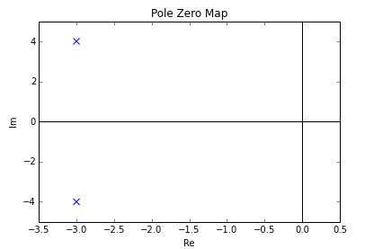Image: Pole–zero plot in the s-plane, CC BY-SA 4.0 — poles marked ×, zeros marked ○.

For $H(s)=N(s)/D(s)$ with both polynomials in $s$:

• Zeros: values of $s$ where $H(s)=0$ — the roots of $N(s)$.
• Poles: values of $s$ where $H(s)\to \infty$ — the roots of $D(s)$.

Why pole locations matter

The poles of $H(s)$ are the eigenvalues of the system’s differential equation — the rates at which the system decays in the absence of input. So they encode every time-domain feature of the impulse response:

• Real part of pole $\sigma$: decay (or growth) rate. Negative $\sigma$ → decaying transient; positive $\sigma$ → growing (unstable).
• Imaginary part of pole ${\omega }_0$: oscillation frequency. Nonzero imaginary part → oscillation.
• Distance from origin $|s|=\sqrt{{\sigma }^2+{\omega }_0^2}$: natural frequency ${\omega }_n$, the speed of the system’s response.
• Repeated poles of order $n$ at $s=\sigma +j{\omega }_0$: bring in the full set of polynomial-times-exponential terms $\{t^k{e}^{(\sigma +j{\omega }_0)t}:k=0,1,\dots ,n-1\}$. The highest-order term $t^{n-1}{e}^{\sigma t}$ dominates at large $t$, but all the lower-order terms appear in the partial-fraction expansion and contribute to the early-time response.

A first-order pole at $s=-1/\tau$ corresponds to a decaying exponential with time constant $\tau$. A pair of complex-conjugate poles at $-\alpha \pm j{\omega }_0$ corresponds to a damped sinusoid $e^{-\alpha t}\cos ({\omega }_{0}t+\varphi )u(t)$.

Stability from poles

For a causal LTI system, BIBO stability requires all poles in the open left half-plane (negative real parts). Poles in the right half-plane → unstable (growing). Simple poles on the imaginary axis → marginally stable (sustained oscillation, neither growing nor decaying). Repeated poles on the imaginary axis → unstable (growing oscillation).

This pole-location criterion is one of the most-used tools in classical control theory and filter analysis.

What zeros do

Zeros don’t determine stability — they don’t appear in the system’s natural response. But they shape the frequency response: at a zero on the imaginary axis $s=j{\omega }_z$, the system completely blocks the frequency ${\omega }_z$. This is how notch filters kill specific frequencies (60 Hz hum, for instance).

In the Bode plot, a zero adds $+20$ dB/decade to the magnitude slope past its corner frequency and adds $+90°$ to the phase; a pole adds $-20$ dB/decade and $-90°$. Zeros and poles “cancel” each other when they’re close, and the spacing between them shapes the rolloff.

Pole-zero plot

A pole-zero plot is just a sketch of the s-plane with poles marked as × and zeros as ○. From the plot you can read off the system’s behavior at a glance:

• All בs in the left half-plane → stable.
• Any × on or right of the imaginary axis → unstable or marginally stable.
• ○ at $s=0$ → DC zero (signal is “AC-coupled” through this system).
• ○ near a ×: zero-pole cancellation; the corresponding mode is mostly suppressed.

Filter design language

Filter design becomes the engineering art of placing poles and zeros on the s-plane to get a desired frequency response. Different filter families (Butterworth, Chebyshev, Elliptic) correspond to different pole/zero placement strategies. The trade-offs are between passband flatness, transition bandwidth, stopband attenuation, and order. See Filter (signal processing).