The BJT small-signal model is the linear equivalent circuit you substitute for a BJT after its DC operating point is known, to analyse how it responds to small AC signals. It comes from linearising the exponential large-signal model around the bias point, the same Small-signal model workflow used for the MOSFET.
The four parameters
Every active-mode BJT small-signal model is built from these, all evaluated at the DC operating point:
| Parameter | Formula | Meaning | Typical at , |
|---|---|---|---|
| transconductance, output current per input voltage | 40 mA/V | ||
| input resistance looking into the base | 2.5 kΩ | ||
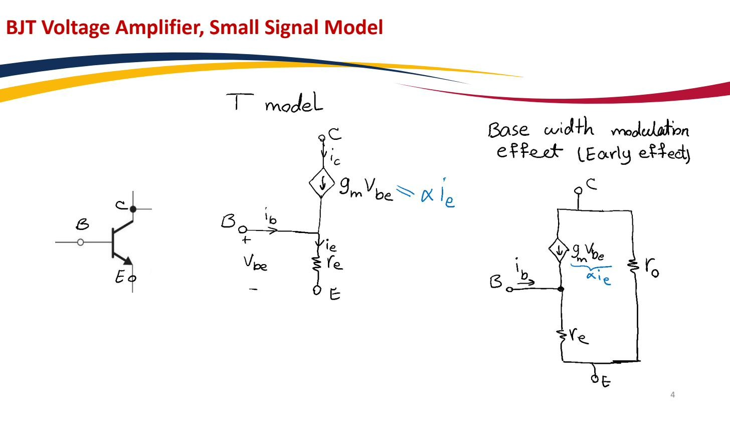
| emitter resistance looking into the emitter | ≈ 25 Ω | ||
| output resistance from the Early effect | ≈ 100 kΩ () |
Here is the Thermal voltage, the Common-emitter current gain, the Common-base current gain, and the Early voltage. These four numbers fully describe the active-mode BJT for small signals; everything else is circuit topology around them. They’re related: , the Resistance reflection rule applied to the device itself.
 The parameters that fully describe the BJT in active mode: , , , and .
Two equivalent representations
The same physics is drawn two ways; both give identical answers, so pick whichever makes the circuit easier:
- The BJT hybrid-pi model puts between base and emitter and the controlled source between collector and emitter. Convenient when the base is the input node, i.e. Common-emitter amplifier and Emitter follower.
- The BJT T-model puts between base and emitter (carrying the full emitter current). Convenient when the emitter is the signal node, i.e. Common-base amplifier and emitter-follower output-resistance calculations.
The model is valid only in active mode and only for signals small enough that the linearisation holds (the discarded quadratic term in the BJT transconductance expansion stays negligible). For DC/large-signal work, go back to the BJT large-signal model.